The Orthopolity cosmological principle and the Natural distribution law
Abstract
Orthopolity is a third cosmological principle, together with Isotropy and Homogeneity. From it, we derive the Natural distribution law. Orthopolity is the equal distribution of resources along unit load: more resources on the unit makes it less frequent. The Natural Distribution Law, where the frequency of a container load is inversely proportional to its quantity of resources, yields a power law.
Introduction
Things tend to be more numerous when the conditions for it abound. One may argue that, of course, if there is space for more, there will be a tendency for it be more. And it is true, and the consequences of this simple observation are profound and yield a ubiquitous natural law. For example: there are more buttons in your computer than screens, more flies than elephants, more bits than bytes stored in one device.
It follows that when the medium in which the units exist does not impose restrictions, the distribution tends to follow a power law. There are many models and theories on why it is so. Here I argue, with simple geometric and algebraic arguments, that it is a Natural Law on its own, steeming from the fact that in this universe there are things and quantities. I also provide a computer model and tools to observe the phenomenon and its mathematical consequences.
One of these things to be observed is that in real systems the medium imposes itself, constructing the power law. The medium’s restrictions and non-linearities may in fact distort the power-law, and often does it. You can think of this distortion as being caused by some sort of “friction”, and the distortion itself being a “friction coefficient function”. Examples:
- Zipf’s law where the number of short words (and more frequent words) is restricted e.g. by phonetic diversity. More on this later.
- Air trafic might get difficult to handle in airports if there are too many flights. Also: if an airport has too few flights, it might cease to exist.
- When its crowded, more people makes it more difficult to move around, preventing more people from coming in.
- Extremes often yield restrictions, and distort the power law. Pareto, for example, is defined as the power-law with a cutoff of \(x > x_{min}\).
- When there is an optimum quantity for the container, the distribution tends to have a peak, often leading to the bell curves seen for example in height and weight of specific species.
- When many probability distributions are summed, the result is a normal distribution, as seen in the central limit theorem.
A geometric representation of this natural law is based on things, or boxes, in one big thing, or a bigger box. Consider your house or your building or neighborhood. There are many things in it, many rooms, many people, many insects, many unicelular organisms, etc. The smaller these things are, the more of them you tend to have, i.e. the more they tend to be frequent. See section “Intuition” for more examples.
Is nature respecting some sort of minimum action principle again?
Nomenclature
\(u\) is a unit, a container, \(u_i\) is unit i, \(U=\{u_i\}_1^N\) is the set of all N units in consideration. Think of \(u\) as a room, a person, a city, a country, a planet, a star, a galaxy, a universe, a word, an idea, a tecnological device, etc.
\(r\) is a resource, \(r_j\) is resource j, \(R=\{r_j\}_1^M\) is the set of all M resources in consideration. Think of \(r\) as space, time, information, food and water, air, light, matter, power, knowledge, health, war, money, etc.
\(q(i, j) = u_i(r_j)\) is the quantity of resource \(r_j\) in unit \(u_i\).
\(m(j, i) = r_j(u_i)\) is the quantity unit \(u_i\) holds of resource \(r_j\).
Thus, \(q(i, j) = m(j, i) = u_i(r_j) = r_j(u_i)\).
We can also define \(q(I, J)\) as an abstract totality (or total quantity) of a resources available (or allocated), \(q(i,J)\) as the quantity of all resources unit \(u_i\) has, \(q(I,j)\) as the quantity of resource \(r_j\) all units have.
One might probably remove \(u\) and \(r\) altogether and work the algebra with \(q\), \(i\), and \(j\) only. The variables \(u\) and \(r\) are useful in order to address them in the diversity they might hold. The universe or system considered might have units \(u_1\) and \(u_2\) subtantially different. The same goes for resources \(r_1\) and \(r_2\).
The equivalence on \(q\) and \(m\) is meant to make explicit the simplicity of the model and the description given here. It also makes evident further routes to analyse and model the system, e.g. one may address \(n(i, j)\) as the fraction of the resource \(j\) in \(u_i\).
Postulates or Assumptions
1)
If the resource r(u) can be quantified, the more resource r(u) a unit u has, the less frequent (or improbable) p(u). In general terms:
\(p(u) \propto F(1 / r(u)) \propto F(c * [r(u)] ^ {-\alpha}) \propto F(b + c * [r(u)] ^ {-\alpha})\).
Notice that \(b\) might be considered an intrinsic resource that the unit has on its own (and that \(b_i\) the intrinsic resource of unit \(u_i\)), not considered in the term of resources distributed: \(c * [r(u)] ^ {-\alpha}\). Greater \(b_i\) is more frequent, more probable. Greater \(b\) means the power law term (\(c * [r(u)] ^ {-\alpha}\)) has less influence in the probability.
2) The postulate 1) holds even if the resource r(u) is multidimensional and nonlinear.
Moreover, it can be overuled by some or many other factors and constraints,
but there is a tendency for the power law to be observed.
The postulate 1) yields a natural law, and the deviations from it are the result of other natural laws.
The apple can get stuck in the tree after you throw it up: gravity is acting and it does not fall,
i.e. the natural law of gravitation is acting even if we don’t measure the apple falling down.
3) The \(\alpha\) is related to how rare or valuable is the resource in which \(u\) is embedded, the scale and limits of vality of the power law. At a first glance, larger \(\alpha\) means fewer inviduals exist that hold plenty of the resources and thus the population is skewed to the majority of the population having very little. In a second glance, the limits \(r_{min}\) and \(r_{max}\), but also \(c\) (and \(b\)) influence the value of \(\alpha\). See the apendix of the article in the “Previous work” section for more information.
4) In real systems, the final resource represented through \(r\) is often compound, meaning that more than one resource is being used. The way these resources relate to each other yield 1) the value of \(\alpha\) and 2) deviations from the power law. One useful interpretation of \(\alpha\) is the dimensionality of \(r\), as in the boxes in the next section, where \(r\) is the side of the box and \(\alpha = 3\) because the resource is the volume.
Now, let’s explore these postulates in some generic systems, keen to many other systems, real or ideal.
Intuition
Ideal Boxes
Ideal boxes fit perfectly together, leaving no space between them, and can have fractional sizes.
Consider a square box with side of length \(l\).
The volume of the box is \(l^3\).
Consider a greater square box with side of length \(L\).
You can fit \(L^3/l^3\) boxes in the greater box.
The smaller the box, the more you can fit in the greater box.
This translates into more things of smaller size (probably) existing in your house or in your city, for example.
See the picture for size propability from 1m to 10m in a larger box with \(L=100m\):
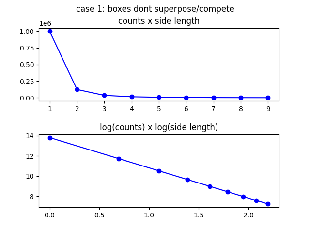
The perfect line in the log x log plot is due to the power law. Now lets understand why it is not perfectly a power-law distribution in the case of your body or house or your city.
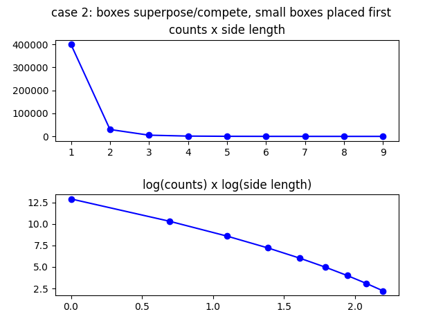
Supose you now have boxes of length \(l_i\) and will fit them in the greater box,
but boxes cannot be inside one another.
At each box size, a fraction \(\epsilon\) of the empty space is filled with boxes of that size,
You can interate from the smallest to the largest box, or from the largest to the smallest box.
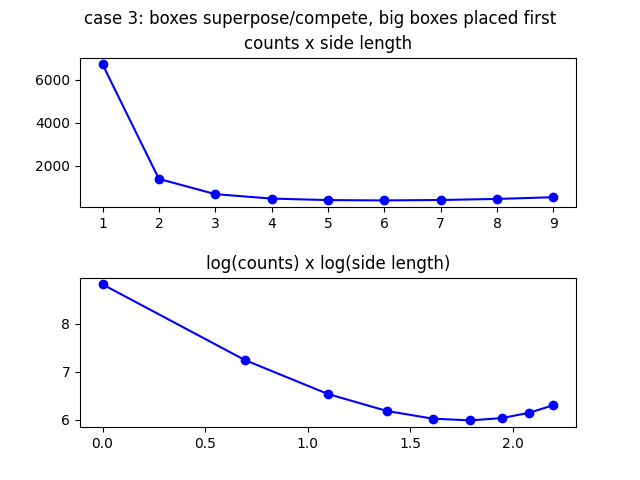
Next you see the picture for both cases, where \(L=100\), \(l=1...9\), and \(\epsilon=0.4\).
Notice the deviation from the straight line in the log x log plots.
Prioritizing the smaller boxes:
Prioritizing the larger boxes:
Sound on frequency, cycles, periods, wavelengths
Consider a real sound, it typically has many frequencies, or oscillatory components. Frequencies don’t compete, i.e. two frequencies can exist at the same time and space. You can think about it a special case of the (ideal) boxes, in which they exist in one dimension and can be superposed.
If a cycle of an oscillation takes long, there are less cycles in a given duration. This is expressed in the known relation between frequency and period:
\[f = 1 / T\]That is, the less time (resource) an oscillation takes, the more you have of it.
Now supose your sound is traveling a medium with constant \(v\). You know that speed is \(v = \lambda * f\) where \(\lambda\) is the wavelength. Finally, observe that:
\(f = v / \lambda\).
The relations for \(f\) with \(T\) and \(\lambda\) are cases of pure orthopolity, in which the medium in which they exist does not impose restrictions for them to coexist (nor competition mechanisms).
Words in a language
Words (in a language or corpus) follow the Zipf’s law:
\[f \propto r^{-\alpha}\]where \(f\) is the frequency of the word, \(r\) is the rank of the word. Deviations are reported to respect a constant in the rank variable: \(f \propto (r + b)^{-\alpha}\) (with \(\alpha\) is typically \(\approx 1\)), the Zipf-Mandelbrot law, and also are found to produce quasi-Zipfian distributions is some time-dependant corpora.
Steven’s law (and Weber-Fechner law)
The intensity of the stimulus \(I\) is related to the magnitude of its sensation \(\Psi(I)\) through: \(\Psi(I) = k * I^{-\alpha}\) which is a power law with \(\alpha\) typically in \([-2, -0.3]\).
Is this power law an evidence of orthopolity or \(I\) and \(\Psi(I)\) don’t relate as “quantities” in “containers”?
The Weber-Fechner can be related to a power law through: https://en.wikipedia.org/wiki/Pareto_distribution#Relation_to_the_exponential_distribution
People in a city
There are incoveniences in having too many people in a city. But the advantages seem to balance it out because it follows a power law quite well: https://www.researchgate.net/figure/Observed-and-estimated-numbers-of-cities-and-average-city-populations-in-different-city_fig1_265034264
People and knowledge
Consider that if a person \(u_i\) spends an hour in one activity/subject \(r_j\), such a person has one hour of knowledge about activity \(r_j\). Consider that there is no limit in the quantity a person can accumulate of hours (of knowledge). And that the knowledge that one person has is (ideally) not limited by the knowledge other people have.
Thus we should expect a power-law distribution of knowledge (of a specific activity/subject \(r_i\) or about a set of them \(\{r_i\}\)) among people. And we should expect deviations from the power law because there are many restrictions and influences of the medium in which the knowledge is acquired and shared. For example knowledge about one subject/activity influences the others (e.g. if you know a lot about civil engineering, you might know a lot about architecture, for example). Also the number of hours a person have is limited, life changes and so the activities, etc.
You might observe that, related to knowledge, you have very few leading references, a number of specialists, and a lot (a lot) of people that know a little about the subject. As expected by the power law.
Equality of resources distributed, inequality of resources hold
Consider \(p(k) = C * k^{-\alpha}\), where \(p(k)\) is the probability of a unit having resource with parameter \(k\). Now, the propability of such a person existing in a population of \(N\) people is: \(P(k) = N * p(k) = N * C * k^{\alpha}\). The quantity of resources held by people with \(k^{\alpha}\) resources (i.e. \(k\) resources with dimensionality \(\alpha\)) is: \(Q(k) = N * k^{\alpha} * p(k) = N * C = C'\) which is constant.
That is, be \(k_1 \neq k_2\) and \(k\) discrete:
\(Q(k_1) = Q(k_2) = C'\), which expresses the orthopolity principle.
Exercise: what happens when k is continuous?
Conclusions
The power-law distribution is a “Natural Distribution”, sister to the Normal distribution to which it contrasts. It is the outcome of the Orthopolity cosmological principle, brother to the Isotropy and Homogeneity cosmological principles.
The observation of this principle and of this law, as characteristics of this universe, changes:
- The way we think about, simulate, and analyse the universe and its systems.
- The way we think about, simulate, and analyse the data we have about the universe and its systems.
- The way we think about, simulate, and analyse the models we have about power laws and related phenomena. For example: the “rich get richer” (a.k.a. “preferential attachment” in network theory) model might not be seen as the generating model for a power law, but as a model that copes with nature because it respects the orthopolity principle. There are, in facts, many other mechanisms in action in a system, beyond the “rich get richer”, many of them generating (or favoring) power law distributions and many generating other distributions.
- How we view equality and inequality in human society and the rest of nature. In fact, the last section ephasizes this point.
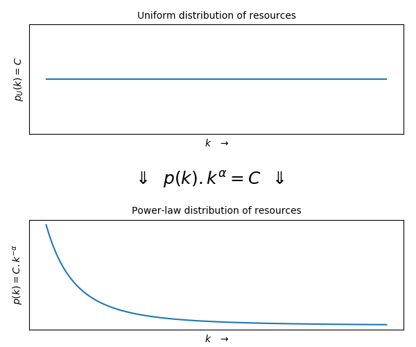
Uniform(k) => Power(k)
One of the most impressive consequences of orthopolity is that the uniform distribution of resources yields a power law distribution of resources.
The uniform distribition is that of resources among the concentration of it in containers, which can be expressed with \(p(k) * k^{-\alpha} = C\). This means that the same amount of resources is allocated to the countainers that have little and to the containers that have a lot of resources, and this is reflected in the fewer containers that have a lot of resources.
The power law distribution is that of resources among containers, which can be expressed with \(p(k) = C * k^{-\alpha}\). The first equation conveys the orthopolity principle, the second is the natural distribution law:
Further work
https://www.investopedia.com/terms/i/isoquantcurve.asp
Previous work
https://zenodo.org/records/3973549
Scripts and tools
I hope to make a library to explore the models and also relations among \(p(k)\), \(\alpha\), \(c\), \(k_l\), \(k_r\). And also how they relate to mean, variance, median, etc. Some scripts are already available at: https://github.com/1etteratura/1etteratura.github.io